12 Introduction to R and RStudio
12.1 Introduction
Importance of R in Mass Communications
The Changing Landscape of Media and Communication
In the evolving landscape of media and communication, traditional skills in writing, editing, and reporting are no longer sufficient. In our data-driven society, quantitative reasoning and data manipulation are becoming increasingly crucial competencies (Couldry & Turow, 2014).
Computational Journalism and Data-Driven Storytelling
The emergent field of computational journalism utilizes algorithms and data analytics to generate stories or insights (Diakopoulos, 2019). For instance, data-driven journalism may involve scrutinizing social media trends or analyzing large data sets to unearth patterns relevant to public interest.
Audience Analytics and Consumer Behavior
Understanding your audience is critical in mass communications. R provides powerful tools for analyzing consumer behavior and audience engagement, helping organizations to optimize their content strategy and even predict future trends (Chaffey & Smith, 2017).
What is R and RStudio?
R: More Than Just a Statistical Package
At its core, R is a programming language designed for statistical analysis and visualizing data. However, its capabilities extend far beyond this. Libraries like ggplot2 for data visualization, tidytext for text mining, and lubridate for handling date-times enable a broad spectrum of functionalities (Wickham & Bryan, 2011; Silge & Robinson, 2016; Grolemund & Wickham, 2011).
## [1] 3RStudio: The Integrated Development Environment
RStudio acts as a centralized platform that makes the usage of R more efficient and accessible. RStudio provides various panes for different tasks: a console for running code, a script editor for saving and editing scripts, an environment pane that shows all your current variables, and a viewer for plots and other outputs.
# Sample R code executed in RStudio to plot a simple graph
x <- seq(1, 10, 1)
y <- x^2
plot(x, y, main = "A Simple Plot")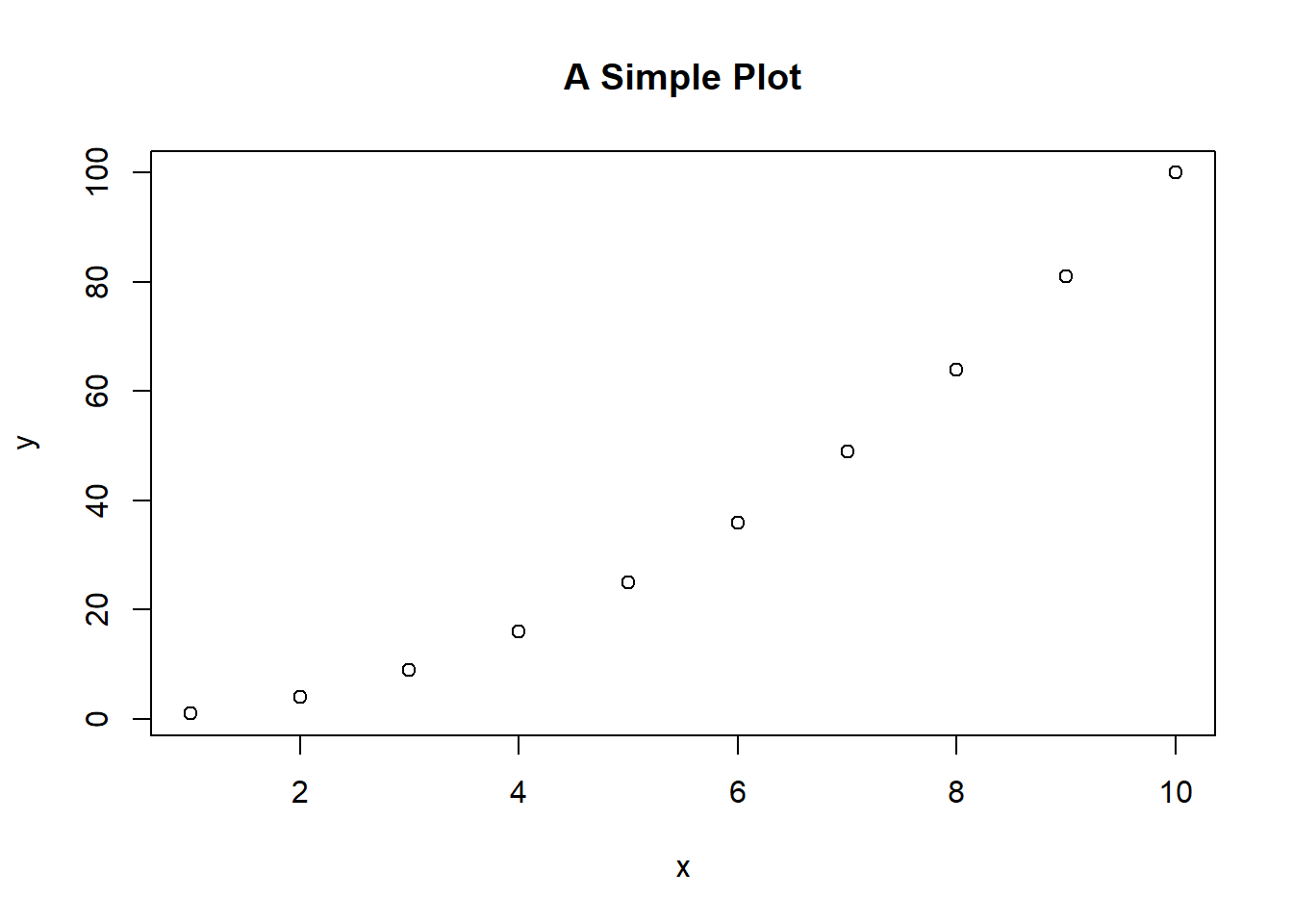
R Markdown
One significant feature in RStudio is the R Markdown tool, which allows you to integrate code, outputs, and narrative text in a single document. This is particularly useful for creating reports, articles, or even interactive web pages (Xie, Allaire, & Grolemund, 2018).
# Sample R Markdown code chunk to display a table

data <- data.frame(Name = c("Alice", "Bob"), Age = c(30, 40))
knitr::kable(data)| Name | Age |
|---|---|
| Alice | 30 |
| Bob | 40 |
12.2 Understanding the Basics
Open Source Software
The Open-Source Philosophy
Open-source software is based on the principle that the source code of a program should be made publicly available. This allows anyone to view, modify, and distribute the code, offering several advantages, including transparency, community development, and flexibility (Stallman, 2002).
Advantages for Academic Research
In the academic setting, the open-source nature of R and RStudio makes them particularly appealing for research. Transparency in the code aids in the reproducibility of research findings, a key criterion for academic rigor (Peng, 2011).
Customizability and Extensibility
The open-source nature also means that you can tailor R to suit your specific research or project needs. For example, if R does not natively support a particular type of analysis, you can write your own functions to perform this analysis.
# Example of creating a simple function to calculate the square of a number
square_function <- function(x) {
  return(x * x)
}

# Using the function
square_function(5)  # Output will be 25
## [1] 25Community Support
Vibrant Ecosystem
The active community around R and RStudio is one of their most robust features. Developers and users contribute to a constantly growing repository of packages, which extend the basic functionalities of R to areas like advanced statistical modeling, natural language processing, and network analysis (Csardi & Nepusz, 2006; Feinerer, Hornik, & Meyer, 2008).
Package Maintenance and Updates
The community’s active involvement also means that packages are regularly updated to include new features, fix bugs, and improve performance. This ensures that you have access to cutting-edge tools and methodologies for your work in communications and media.
12.3 Installing R and RStudio
Installing R
The installation of R serves as a pre-requisite to utilizing RStudio, as the latter is essentially an IDE built on top of the R environment. Below are detailed steps for installing R on Windows and macOS systems.
Windows
Step-by-Step Instructions
Visit the Comprehensive R Archive Network (CRAN) Website: Navigate to the CRAN repository at https://cran.r-project.org/.
Select the Appropriate Version for Windows: Click on the link titled “Download R for Windows”. On the next page, click “install R for the first time” followed by “Download R x.x.x for Windows”, where x.x.x is the latest version number.
Run the Installer: Locate the downloaded
.exefile (usually in theDownloadsfolder) and double-click to initiate the installation process.Follow the Prompts: The installation wizard will guide you through several screens where you can select options like the install directory. Default options are generally safe to use.
Note: Administrative rights may be required for installation. If prompted, enter the administrative password or contact your system administrator.macOS
System Requirements
- Operating System: macOS 10.13 (High Sierra) or higher
- Disk Space: Approximately 200MB
Step-by-Step Instructions
Visit the CRAN Website: Go to https://cran.r-project.org/.
Select the Appropriate Version for macOS: Click on the link titled “Download R for (Mac) OS X”. Download the
.pkgfile corresponding to the latest R version.Open the Package: Locate the downloaded
.pkgfile and double-click to initiate the installer.Drag the R Icon: A new window will open displaying the R icon. Drag this into your
Applicationsfolder to complete the installation.
Note: Administrative rights may be necessary for completing the installation on macOS as well. Ensure that you have the necessary permissions.Installing RStudio
With R successfully installed, the next step is to install RStudio, which provides a more user-friendly interface for interacting with R.
Step-by-Step Instructions
Visit the RStudio Website: Navigate to the official RStudio website at https://rstudio.com/products/rstudio/download/.
Download the Installer: Select the installer corresponding to your operating system—either Windows or macOS.
Run the Installer:
-
For Windows: Double-click the downloaded
.exefile and follow the installation prompts. -
For macOS: Double-click the downloaded
.dmgfile. Drag the RStudio icon to yourApplicationsfolder.
- Complete the Installation: Follow the installation wizard’s prompts to complete the installation. Default settings are typically sufficient for most users.
Note: Just like with R, administrative rights may be necessary for the installation of RStudio. Please consult your system administrator if you encounter permission issues.By completing these steps, you will have successfully installed both R and RStudio on your system, laying the foundation for your computational endeavors in mass communications and media research.
12.5 Basic Operations in R
Understanding the basic operations in R is vital for embarking on more complex data analysis and programming tasks. These operations include arithmetic calculations, variable assignments, and function calls.
Arithmetic Operations
Overview
Arithmetic operations form the basis of numerical calculations in R. These operations can be conducted directly in the R console and include addition, subtraction, multiplication, division, exponentiation, and other mathematical functions (Chambers, 2008).
Common Arithmetic Operators
-
Addition (
+): Adds two numbers. -
Subtraction (
-): Subtracts the right-hand operand from the left-hand operand. -
Multiplication (
*): Multiplies two numbers. -
Division (
/): Divides the left-hand operand by the right-hand operand. -
Exponentiation (
^): Raises the left-hand operand to the power of the right-hand operand. -
Modulus (
%%): Gives the remainder of the division between two numbers.
Examples
You can execute these basic arithmetic operations directly in the R console.
Addition
5 + 3## [1] 8Subtraction
5 - 3## [1] 2Multiplication
5 * 3## [1] 15Division
5 / 3## [1] 1.666667Exponentiation
5 ^ 3## [1] 125Modulus
5 %% 3## [1] 2Variables
What Are Variables?
Variables act as storage containers for data, including numbers, strings, vectors, and other complex data types. Variable assignment is a crucial aspect of programming and data management in R (Wickham, 2014).
Functions
Function Overview
Functions are predefined sets of operations that perform specific tasks. Functions in R can be either built-in, such as sum() or mean(), or user-defined for more customized operations (Chambers, 2008).
Built-in Functions
Examples of common built-in functions include:
dz
- sum(): Calculates the sum of all the values in a numeric vector.
- mean(): Calculates the arithmetic mean of a numeric vector.
- sqrt(): Calculates the square root of a number.
Using sum function
sum(1, 2, 3)## [1] 6Using mean function
## [1] 2.5Using sqrt function
sqrt(16)## [1] 4User-Defined Functions
You can also create your own functions in R. These are particularly useful for tasks that you plan to repeat often.
# Defining a function to calculate the square of a number
square_number <- function(x) {
  return(x * x)
}

# Using the function
square_number(4)
## [1] 16By understanding the basics of arithmetic operations, variable assignment, and function usage, you can lay a strong foundation for more complex statistical analyses and computational research in mass communications.
12.6 Data Structures in R
Data structures are fundamental in R programming as they organize and store the data that one works with for analyses, visualizations, and other computational tasks. Understanding these structures is critical for effective manipulation of data and implementing various algorithms (Wickham & Grolemund, 2017). Below are the primary data structures that R provides.
Vectors
Overview
Vectors are one-dimensional arrays used to hold elements of a single data type. This could be numeric, character, or logical data types. Vectors are often used for operations that require the application of a function to each element in the data set (Maindonald & Braun, 2010).
Creating Vectors
Vectors can be created using the c() function, which combines elements into a vector.
Matrices
Overview
Matrices are two-dimensional arrays that hold elements of the same data type. They are used in various applications, including image processing, linear algebra, and statistical analyses (Ripley, 2001).
Creating Matrices
Matrices can be created using the matrix() function.
Data Frames
Overview
Data frames serve as the fundamental data structure for data analysis in R. They are similar to matrices but allow different types of variables in different columns, which makes them extremely versatile (Chambers, 2008).
Creating Data Frames
Data frames can be created using the data.frame() function.
Examples
# Creating a data frame
df <- data.frame(Name = c("Alice", "Bob"), Age = c(23, 45), Gender = c("F", "M"))
Operations on Data Frames
Various operations like subsetting, merging, and sorting can be performed on data frames.
# Subsetting data frame by column
subset_df <- df[, c("Name", "Age")]
Lists
Overview
Lists are an ordered collection of objects, which can be of different types and structures, including vectors, matrices, and even other lists (Wickham & Grolemund, 2017).
Creating Lists
Lists can be created using the list() function.
Operations on Lists
Lists can be modified by adding, deleting, or updating list elements.
# Updating a list element
my_list$Name <- "Bob"

# Adding a new list element
my_list$Email <- "bob@email.com"
By understanding these primary data structures, students in Mass Communications can gain a strong foundation for more complex data analyses relevant to their field, whether it involves analyzing large sets of textual data, audience metrics, or other forms of media data.
12.7 Installing and Loading Libraries
Libraries, or packages as they are often called, are bundles of pre-written code that provide additional functionality to the base R environment. In the realm of mass communications, these packages can extend R’s capabilities to perform tasks like text analysis, social network analysis, and even web scraping (Cranefield & Yoong, 2007; Lewis, Zamith, & Hermida, 2013). As a result, understanding how to install and load libraries is a fundamental skill.
Installation
Overview
The installation process essentially adds the package files to your R environment, making it possible for you to use the package’s built-in functions, data sets, and other utilities (Wickham & Grolemund, 2017).
Installing from CRAN
The Comprehensive R Archive Network (CRAN) serves as the primary repository for R packages. The following command installs a package from CRAN:
# To install the ggplot2 package
# install.packages("ggplot2", repos = 'http://cran.us.r-project.org')
Installing from GitHub
Sometimes, packages may not be available on CRAN and could be hosted on other platforms like GitHub. The devtools package allows you to install these:
# First install devtools if you haven't
# install.packages("devtools", repos = 'http://cran.us.r-project.org')

# Use devtools to install a package from GitHub
# devtools::install_github("username/package_name")
Dependencies
Some packages depend on other packages to function correctly. Usually, dependencies are automatically installed, but you can ensure this by setting the dependencies argument to TRUE.
# To install ggplot2 along with its dependencies
# install.packages("ggplot2", dependencies = TRUE, repos = 'http://cran.us.r-project.org')
Loading
Overview
Once installed, a package must be loaded into the current R session to utilize its functions. This is a crucial step; otherwise, attempts to use the package’s functions will result in errors (Wickham, 2015).
Loading a Package
You can load an installed package using the library() function:
Unloading a Package
To unload a package, you can use the detach() function:
# To unload the ggplot2 package
detach("package:ggplot2", unload=TRUE)
Checking Loaded Packages
To check which packages are currently loaded in the session, you can use the sessionInfo() function:
# To get information about the session, including loaded packages
sessionInfo()
## R version 4.3.2 (2023-10-31 ucrt)
## Platform: x86_64-w64-mingw32/x64 (64-bit)
## Running under: Windows 11 x64 (build 22621)
##
## Matrix products: default
##
##
## locale:
## [1] LC_COLLATE=English_United States.utf8
## [2] LC_CTYPE=English_United States.utf8
## [3] LC_MONETARY=English_United States.utf8
## [4] LC_NUMERIC=C
## [5] LC_TIME=English_United States.utf8
##
## time zone: America/Chicago
## tzcode source: internal
##
## attached base packages:
## [1] stats graphics grDevices utils datasets methods base
##
## loaded via a namespace (and not attached):
## [1] vctrs_0.6.4 cli_3.6.1 knitr_1.45 rlang_1.1.2
## [5] xfun_0.41 highr_0.10 generics_0.1.3 jsonlite_1.8.7
## [9] glue_1.6.2 colorspace_2.1-0 htmltools_0.5.7 sass_0.4.7
## [13] fansi_1.0.5 scales_1.2.1 rmarkdown_2.25 grid_4.3.2
## [17] tibble_3.2.1 munsell_0.5.0 evaluate_0.23 jquerylib_0.1.4
## [21] fastmap_1.1.1 yaml_2.3.7 lifecycle_1.0.4 memoise_2.0.1
## [25] bookdown_0.36 compiler_4.3.2 dplyr_1.1.4 fs_1.6.3
## [29] pkgconfig_2.0.3 downlit_0.4.3 rstudioapi_0.15.0 digest_0.6.33
## [33] R6_2.5.1 tidyselect_1.2.0 utf8_1.2.4 pillar_1.9.0
## [37] magrittr_2.0.3 bslib_0.6.0 tools_4.3.2 withr_2.5.2
## [41] gtable_0.3.4 xml2_1.3.5 cachem_1.0.8Understanding the installation and loading process for libraries will enable you to extend R’s native functionalities, a vital skill in today’s data-driven landscape in mass communications.
12.8 Creating and Managing Projects
In the realm of mass communications research and practice, a multitude of projects often run concurrently, whether it’s data analysis for audience segmentation, sentiment analysis for social media content, or exploratory research in emerging media technologies. Thus, the ability to efficiently manage these projects is crucial. RStudio provides an intuitive way to create and manage projects, thereby organizing your work effectively (RStudio Team, 2020).
New Projects
Overview
Creating a new project in RStudio essentially initializes a new workspace—a dedicated folder in which R scripts, data files, and other essential resources can be stored (Wickham, 2015).
Steps to Create a New Project
Launch RStudio: If RStudio isn’t open, launch the application.
-
Navigate to New Project:
- Go to the RStudio menu.
- Select
Fileand thenNew Project. This will open a dialog box.
-
Select Project Type:
- You can choose to start a new directory, create a project in an existing directory, or even check out a project from a version control repository like Git.
-
Configure Options:
- Name your project.
- Choose the directory where it will reside.
- If you want version control, you can initialize a Git repository.
Create Project: Once configured, click
Create Projectto initialize the new workspace.
Here is a conceptual demonstration of how to initialize a new project:
# This is a conceptual code snippet and won't execute
# Navigate to File -> New Project in RStudio
# Choose project type and directory
# Name your project "My_Comm_Project"
# Optionally, initialize a Git repository
# Click "Create Project"
Existing Projects
Overview
Working on existing projects is equally straightforward. Each RStudio project has an associated .Rproj file that stores metadata and settings for that project (Wickham, 2015).
Steps to Open an Existing Project
Launch RStudio: If it is not already open, launch the RStudio application.
-
Navigate to Project File:
- Use your operating system’s file explorer to navigate to the folder containing the
.Rprojfile. - Double-click on the
.Rprojfile to open the project in RStudio.
OR
- Within RStudio, go to
File -> Open Projectand navigate to the.Rprojfile.
- Use your operating system’s file explorer to navigate to the folder containing the
Here’s a conceptual guide to open an existing project:
# This is a conceptual code snippet and won't execute
# Navigate to File -> Open Project in RStudio
# Browse to locate your .Rproj file, e.g., "My_Old_Comm_Project.Rproj"
# Click "Open"
Understanding how to create and manage projects in RStudio is pivotal for structured and efficient work, especially in the complex and multifaceted landscape of mass communications.
Exhaustively expand the following sections with consideration for this being an upper-level undergrad textbook for communication and media students. Please include code examples when relevant. For code examples, do not require external data or sources.
12.9 Summary
This chapter provides a foundational understanding of R and RStudio, equipping mass communications students with the basic skills to navigate and utilize these tools for more advanced, discipline-specific applications in subsequent chapters.
12.10 References
Borgatti, S. P., Everett, M. G., & Johnson, J. C. (2013). Analyzing social networks. SAGE Publications Limited.
Chaffey, D., & Smith, P. R. (2017). Digital marketing excellence: Planning, optimizing and integrating online marketing. Routledge.
Chambers, J. M. (2008). Software for Data Analysis: Programming with R. Springer.
Couldry, N., & Turow, J. (2014). Advertising, big data and the clearance of the public realm: Marketers’ new approaches to the content subsidy. International Journal of Communication, 8, 17.
Cranefield, J., & Yoong, P. (2007). Cross-disciplinary research in the creation of a computational toolkit for collaborative learning in the social sciences. Journal of Information Technology Education: Research, 6(1), 67–82.
Csardi, G., & Nepusz, T. (2006). The igraph software package for complex network research. InterJournal, Complex Systems, 1695(5), 1-9.
Diakopoulos, N. (2019). Automating the news: How algorithms are rewriting the media. Harvard University Press.
Feinerer, I., Hornik, K., & Meyer, D. (2008). Text mining infrastructure in R. Journal of Statistical Software, 25(5), 1-54.
Grolemund, G., & Wickham, H. (2011). Dates and times made easy with lubridate. Journal of Statistical Software, 40(3), 1-25.
Lewis, S. C., Zamith, R., & Hermida, A. (2013). Content Analysis in an Era of Big Data: A Hybrid Approach to Computational and Manual Methods. Journal of Broadcasting & Electronic Media, 57(1), 34–52.
Maindonald, J., & Braun, J. (2010). Data Analysis and Graphics Using R. Cambridge University Press.
Morin, A., Urban, J., & Sliz, P. (2012). A quick guide to software licensing for the scientist-programmer. PLoS Computational Biology, 8(7), e1002598.
Peng, R. D. (2011). Reproducible research in computational science. Science, 334(6060), 1226-1227.
Ripley, B. D. (2001). The R project in statistical computing. MSOR Connections, 1(1), 23–25.
RStudio Team (2020). RStudio: Integrated Development for R. RStudio, PBC.
Silge, J., & Robinson, D. (2016). tidytext: Text mining and word processing in R. R package version, 0(1).
Smith, A. M., Katz, D. S., Niemeyer, K. E., & FORCE11 Software Citation Working Group. (2018). Software citation principles. PeerJ Computer Science, 2, e86.
Stallman, R. (2002). Free Software, Free Society: Selected Essays of Richard M. Stallman. GNU Press.
Wickham, H. (2014). Advanced R. CRC Press.
Wickham, H. (2015). R packages: organize, test, document, and share your code. O’Reilly Media, Inc.
Wickham, H., & Bryan, J. (2011). readxl: Read Excel files. R package version 1.3.1.
Wickham, H., & Grolemund, G. (2017). R for data science: Import, tidy, transform, visualize, and model data. O’Reilly Media.
Xie, Y., Allaire, J., & Grolemund, G. (2018). R Markdown: The definitive guide. CRC Press.