13 Data
13.1 Defining Data?
Explanation of Data in the Context of Research
In the realm of academic research, data can be broadly defined as a collection of facts, statistics, or observations represented in various forms, such as numbers, text, or images. Data serves as the empirical foundation upon which hypotheses can be tested, theories can be validated, and meaningful insights can be drawn. For researchers in the field of Communication and Media Studies, data might include viewer ratings for television shows, text from social media posts, or timestamps indicating when a user interacted with a media platform, among other examples (Neuendorf, 2016).
Types of Data: Qualitative vs. Quantitative
Data is often classified into two overarching categories: qualitative and quantitative.
Qualitative Data: This type of data is often textual or visual and is used to capture non-numerical information. In the context of the
spotify_songsdataset, qualitative data might include variables such astrack_nameorplaylist_genre. Qualitative data helps researchers delve into the nuanced meanings and descriptions that numbers cannot capture.Quantitative Data: These are numerical data points that can be measured or counted. In the
spotify_songsdataset, examples of quantitative data would includetrack_popularityortempo. Quantitative data are typically analyzed using statistical methods and are integral for hypothesis testing (Wrench, Thomas-Maddox, Richmond, & McCroskey, 2008).
13.2 Variables and Observations
Define Variables and Observations
In data analysis, “variables” refer to the different aspects or dimensions that data can have, while “observations” refer to individual data points within each variable.
Variables: In the
spotify_songsdataset, variables could includetrack_name,playlist_genre, andtrack_popularity, among others. Each variable represents a specific characteristic that has been observed or measured.Observations: These are the individual entries for each variable. For example, under the variable
track_name, each song title would be an observation. Observations populate the dataset, providing the raw material for analysis.
It’s crucial to understand the variables and observations in your dataset, as they serve as the basic units in your data analysis workflow.
Explanation of Data Types
Understanding data types is crucial for effective data manipulation and analysis in R. Incorrect data types can lead to errors and might produce misleading results. Here are some common data types in R, illustrated with examples from the spotify_songs dataset:
Integers: These are whole numbers, either positive or negative. In the
spotify_songsdataset, a column likeduration_ms(duration in milliseconds) might be an integer.Factors: Factors are categorical variables that can take on a limited number of different values. For instance,
playlist_genrecould be treated as a factor with levels such as “pop,” “rock,” “jazz,” etc.Strings (Character): These are sequences of characters and are often used to represent text. In the
spotify_songsdataset,track_namewould typically be a string.Numeric: These include both integers and floating-point numbers (i.e., numbers with decimals). For example,
tempoin thespotify_songsdataset might be a numeric type.
Knowing the data types of your variables is crucial for performing appropriate analyses and avoiding errors in your R code (Wickham & Grolemund, 2017).
13.3 Collecting Data
Discussion of Primary vs. Secondary Data Collection Methods
Collecting accurate and reliable data is pivotal for generating meaningful research conclusions. Two key types of data collection methods are used in academic research: primary and secondary.
Primary Data: This type of data is collected firsthand by the researcher for a specific research question or purpose. It involves activities like conducting interviews, surveys, observations, or experiments. Primary data is often more time-consuming and costly to collect but allows the researcher to control the variables and conditions under which the data is gathered (Fink, 2013).
Secondary Data: This refers to data that has already been collected by someone else for a different research question or purpose. Researchers use secondary data to gain additional insights or to apply new analytical frameworks to existing data sets. The primary advantage of using secondary data is the speed and cost-effectiveness, but a potential limitation could be the mismatch between the data and the specific research question at hand (Johnston, 2017).
The spotify_songs Dataset as an Example of Secondary Data
The spotify_songs dataset serves as an excellent example of secondary data. It comprises various variables such as track_name, playlist_genre, and track_popularity, among others, that have been previously collected by Spotify for their business analytics or user recommendations. Researchers can use this dataset to answer a myriad of questions about music preferences, playlist creation, or even socio-cultural trends in music consumption. The preexisting nature of this dataset saves researchers the time and resources that primary data collection would require.
13.4 Data Sources
Web Scraping, APIs, and Existing Databases
Data sources can vary widely, and the choice of source often depends on the research question, available resources, and required data types. Here are some commonly used methods:
Web Scraping: This involves programmatically gathering data from websites. While web scraping can be a rich source of qualitative and quantitative data, it requires a good understanding of programming and may pose ethical concerns (Marres & Weltevrede, 2013).
APIs (Application Programming Interfaces): APIs allow for a more structured way to collect data from platforms that offer them. APIs are commonly used for social media platforms like Twitter or services like Spotify, often providing more reliable and easier-to-manage data compared to web scraping (Boyles, 2013).
Existing Databases: Academic databases, government repositories, and other specialized databases provide pre-collected data that can be valuable for research. Examples include the U.S. Census Bureau data, World Health Organization databases, and, in the context of our discussion, Spotify’s publicly available data.
Importance of Credible Data Sources
The credibility of your data source significantly impacts the reliability and validity of your research findings. Unreliable data can not only lead to incorrect conclusions but can also diminish the scholarly impact and credibility of the research. Therefore, it is imperative to choose data sources that are reputable, peer-reviewed when possible, and align with your research objectives (Silverman, 2016).
13.5 Cleaning Data for Visualizations and Analyses
How to Import CSV Files into R
- CSV stands for Comma Separated Values. It is a plain text format with a series of values separated by commas.
- A CSV file is just a text file, it stores data but does not contain formatting, formulas, macros, etc. It is also known as flat files.
Use read.csv from base R
csv1 <- read.csv("https://raw.githubusercontent.com/apleith/apleith.github.io/main/mc451/data/spotify_songs.csv", header=TRUE, stringsAsFactors=FALSE)Use read_csv from readr package
#install.packages("readr")
library(readr)

csv2 <- read_csv("https://raw.githubusercontent.com/apleith/apleith.github.io/main/mc451/data/spotify_songs.csv")
## Rows: 32833 Columns: 23
## ── Column specification ────────────────────────────────────────────────────────
## Delimiter: ","
## chr (10): track_id, track_name, track_artist, track_album_id, track_album_na...
## dbl (13): track_popularity, danceability, energy, key, loudness, mode, speec...
##
## ℹ Use `spec()` to retrieve the full column specification for this data.
## ℹ Specify the column types or set `show_col_types = FALSE` to quiet this message.Use fread from data.table package
#install.packages("data.table")
library(data.table)

csv3 <- fread("https://raw.githubusercontent.com/apleith/apleith.github.io/main/mc451/data/spotify_songs.csv")
How to Import Excel Files into R
- It is a binary file that holds information about all the worksheets in a workbook
- An Excel not only stores data but can also do operations on the data
How to Import SPSS Files into R
- Also a binary format.
- Designed for SPSS
#install.packages("foreign")
library(foreign)

#import SPSS file into R
sav1 <- read.spss("https://github.com/apleith/apleith.github.io/raw/main/mc451/data/ATP%20W90.sav", use.value.label=TRUE, to.data.frame=TRUE)
## Warning in
## read.spss("https://github.com/apleith/apleith.github.io/raw/main/mc451/data/ATP%20W90.sav",
## : Undeclared level(s) 2, 3, 4 added in variable: PERS1_W90## Warning in
## read.spss("https://github.com/apleith/apleith.github.io/raw/main/mc451/data/ATP%20W90.sav",
## : Undeclared level(s) 2, 3, 4 added in variable: PERS11_W90Handling Missing Data
Methods for Dealing with Missing Values in the spotify_songs Dataset
- Read in Data: To read in the necessary web data, you must first load the required packaage and then import the CSV file.
# Check if the package is already installed before trying to install it
if (!"readr" %in% installed.packages()[,"Package"]) {
  install.packages("readr", repos = 'http://cran.us.r-project.org')
}

# Load the package
library(readr)

# Define the raw GitHub URL of the dataset
url <- "https://raw.githubusercontent.com/apleith/apleith.github.io/main/mc451/data/spotify_songs.csv"

# Read the CSV file from the URL
spotify_songs <- read_csv(url)
## Rows: 32833 Columns: 23
## ── Column specification ────────────────────────────────────────────────────────
## Delimiter: ","
## chr (10): track_id, track_name, track_artist, track_album_id, track_album_na...
## dbl (13): track_popularity, danceability, energy, key, loudness, mode, speec...
##
## ℹ Use `spec()` to retrieve the full column specification for this data.
## ℹ Specify the column types or set `show_col_types = FALSE` to quiet this message.Handling missing data is a critical step in the data cleaning process. Missing data can introduce bias or lead to inaccurate inferences. There are several ways to handle missing values:
- Complete Case Analysis: This is the simplest method where you remove observations where any of the variables are missing. However, this method may lead to a loss of valuable data (Rubin, 1987).
spotify_songs_complete <- na.omit(spotify_songs)- Mean/Median/Mode Imputation: Replace the missing values with the mean, median, or mode of that variable. It’s a quick solution but can potentially introduce bias (Little & Rubin, 2002).
##
## Attaching package: 'dplyr'
## The following objects are masked from 'package:data.table':
##
## between, first, last## The following objects are masked from 'package:stats':
##
## filter, lag## The following objects are masked from 'package:base':
##
## intersect, setdiff, setequal, union
spotify_songs <- spotify_songs %>%
mutate(track_popularity = ifelse(is.na(track_popularity), mean(track_popularity, na.rm = TRUE), track_popularity))- Multiple Imputation: More sophisticated than mean imputation, it creates multiple datasets and averages the imputed values (Schafer & Graham, 2002).
##
## Attaching package: 'mice'
## The following object is masked from 'package:stats':
##
## filter## The following objects are masked from 'package:base':
##
## cbind, rbind
imputed_data <- mice(spotify_songs, m=5)##
## iter imp variable
## 1 1
## 1 2
## 1 3
## 1 4
## 1 5
## 2 1
## 2 2
## 2 3
## 2 4
## 2 5
## 3 1
## 3 2
## 3 3
## 3 4
## 3 5
## 4 1
## 4 2
## 4 3
## 4 4
## 4 5
## 5 1
## 5 2
## 5 3
## 5 4
## 5 5## Warning: Number of logged events: 10
spotify_songs_complete <- complete(imputed_data)Data Transformation
dplyr Crashcourse
Certainly, this chapter will walk through the common dplyr commands using pipe (%>%) syntax, employing the movies.csv dataset for demonstration. We will start by loading the necessary libraries and the dataset.
## ── Attaching core tidyverse packages ──────────────────────── tidyverse 2.0.0 ──
## ✔ forcats   1.0.0     ✔ stringr   1.5.1
## ✔ ggplot2   3.4.4     ✔ tibble    3.2.1
## ✔ lubridate 1.9.3     ✔ tidyr     1.3.0
## ✔ purrr     1.0.2
## ── Conflicts ────────────────────────────────────────── tidyverse_conflicts() ──
## ✖ dplyr::between()     masks data.table::between()
## ✖ mice::filter()       masks dplyr::filter(), stats::filter()
## ✖ dplyr::first()       masks data.table::first()
## ✖ lubridate::hour()    masks data.table::hour()
## ✖ lubridate::isoweek() masks data.table::isoweek()
## ✖ dplyr::lag()         masks stats::lag()
## ✖ dplyr::last()        masks data.table::last()
## ✖ lubridate::mday()    masks data.table::mday()
## ✖ lubridate::minute()  masks data.table::minute()
## ✖ lubridate::month()   masks data.table::month()
## ✖ lubridate::quarter() masks data.table::quarter()
## ✖ lubridate::second()  masks data.table::second()
## ✖ purrr::transpose()   masks data.table::transpose()
## ✖ lubridate::wday()    masks data.table::wday()
## ✖ lubridate::week()    masks data.table::week()
## ✖ lubridate::yday()    masks data.table::yday()
## ✖ lubridate::year()    masks data.table::year()
## ℹ Use the conflicted package (<http://conflicted.r-lib.org/>) to force all conflicts to become errors
# Load the dataset
movies <- read.csv("https://raw.githubusercontent.com/rfordatascience/tidytuesday/master/data/2021/2021-03-09/movies.csv")
Certainly, a more extensive exploration of each command is provided below:
1. Select
The select() function allows you to choose specific columns in a dataframe. This function is essential when dealing with large datasets containing numerous variables, and you’re interested in a subset for further analysis.
Example 1: Select only the title, year, and budget columns.
Example 2: Use negative indexing to exclude certain columns.
2. Filter
The filter() function is crucial for subsetting data based on conditional statements. It serves to isolate rows that meet specific criteria, which can be particularly useful for exploratory data analysis or preprocessing data for machine learning algorithms.
Example 1: Filter movies released after 2000 with IMDb ratings above 8.0.
Example 2: Filter movies that passed the Bechdel test.
3. Arrange
The arrange() function sorts data based on one or more variables. It is an essential operation for organizing your data for better readability or analysis.
Example 1: Arrange movies by IMDb ratings in descending order.
Example 2: Arrange movies by year and then by budget.
4. Mutate
The mutate() function is used to create or modify variables. It can be employed to calculate new variables based on existing ones, or for transformations necessary for model building or data visualization.
Example 1: Calculate the earnings by subtracting the budget from the domestic gross.
mutated_movies1 <- movies %>%
  mutate(earning = as.numeric(gsub(",", "", domgross)) - budget)
## Warning: There was 1 warning in `mutate()`.
## ℹ In argument: `earning = as.numeric(gsub(",", "", domgross)) - budget`.
## Caused by warning:
## ! NAs introduced by coercionExample 2: Create a Boolean variable indicating whether the movie has high IMDb ratings (>8).
5. Summarise
The summarise() function allows for the creation of summary statistics from your data. It’s often combined with group_by() for aggregated summaries.
Example 1: Calculate the mean IMDb rating for each decade.
summarised_movies1 <- movies %>%
  group_by(decade_code) %>%
  summarise(mean_rating = mean(imdb_rating, na.rm = TRUE))
Example 2: Count the number of movies that pass and fail the Bechdel test.
6. Group_by
The group_by() function facilitates operations within specific subsets or groups in the data. This function is useful for analyzing data at multiple levels.
Example 1: Group by decade.
Example 2: Group by the outcome of the Bechdel test and decade.
7. Rename
The rename() function changes the names of variables, making them more understandable or suitable for downstream tasks like visualization.
Example 1: Rename intgross to International_Gross.
Example 2: Rename domgross to Domestic_Gross.
8. Transmute
The transmute() function, a specialized variant of mutate(), lets you create new variables while dropping all other variables.
Example 1: Create a dataset with only the title and a new variable ROI (Return on Investment).
transmuted_movies1 <- movies %>%
  transmute(title, ROI = as.numeric(gsub(",", "", domgross)) / budget)
## Warning: There was 1 warning in `transmute()`.
## ℹ In argument: `ROI = as.numeric(gsub(",", "", domgross))/budget`.
## Caused by warning:
## ! NAs introduced by coercionExample 2: Create a dataset with only the title and a Boolean variable indicating high IMDb rating.
transmuted_movies2 <- movies %>%
  transmute(title, is_high_rating = ifelse(imdb_rating > 8, TRUE, FALSE))
Each of these dplyr functions contributes to a robust data wrangling toolbox. The power of dplyr is most evident when these functions are combined to carry out complex data manipulation tasks efficiently.
Outliers and Normalization
Identifying and Treating Outliers in the spotify_songs Dataset
Outliers are data points that are significantly different from most of the other data. They can distort the representation and analysis.
- Identifying Outliers
boxplot(spotify_songs$track_popularity)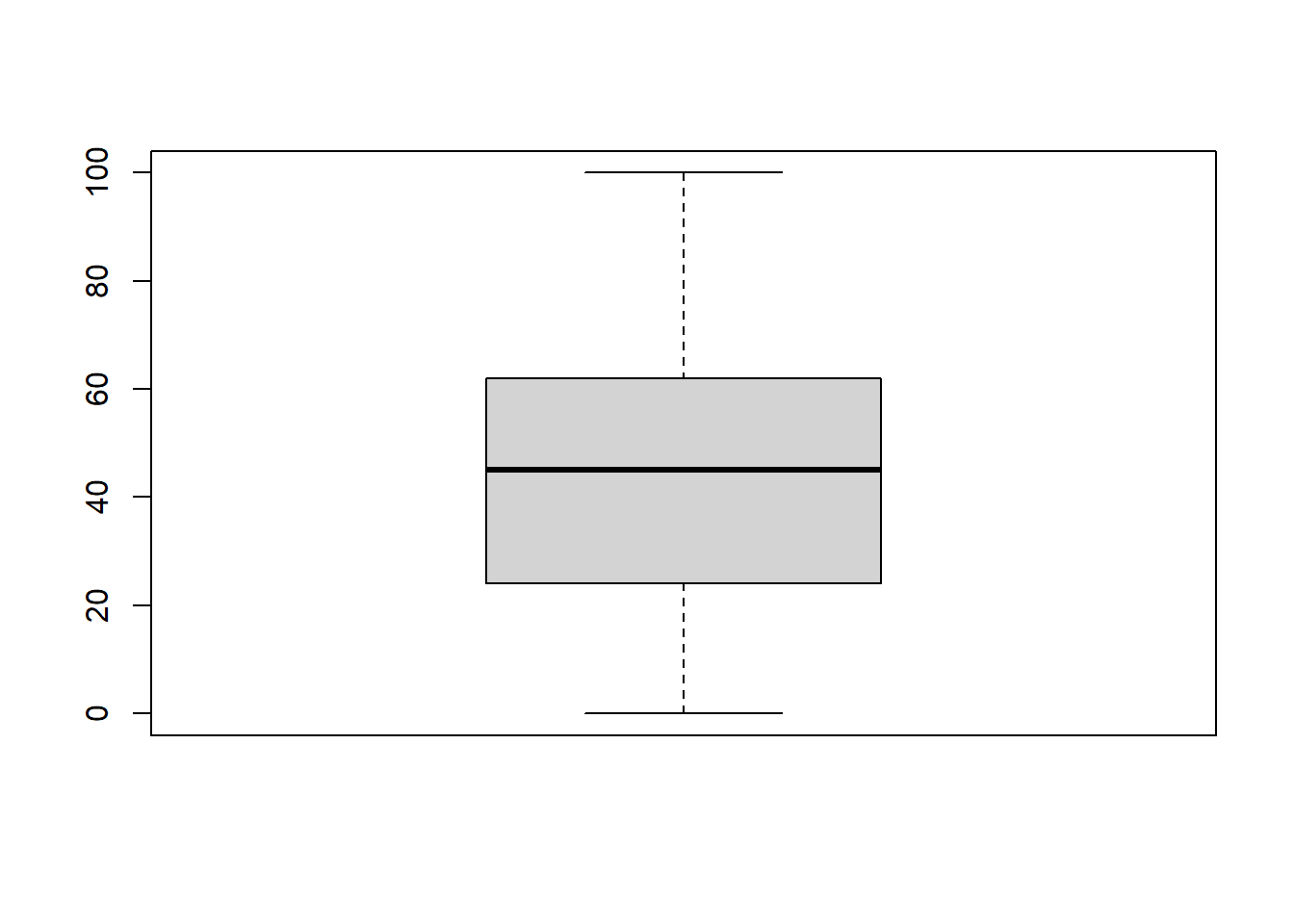
- Treating Outliers: Common methods include transformation, binning, or removing the outliers (Tukey, 1977).
spotify_songs_no_outliers <- filter(spotify_songs, track_popularity < 100)Normalization Techniques
Data normalization is crucial when variables have different scales, as it can bias the results. Common methods include:
- Min-Max Scaling
spotify_songs$normalized_popularity <- (spotify_songs$track_popularity - min(spotify_songs$track_popularity)) / (max(spotify_songs$track_popularity) - min(spotify_songs$track_popularity))- Z-score Normalization